ARIMA stands for AutoRegressive Integrated Moving Average and is a popular time series forecasting model used in statistics and econometrics. This modeling approach is particularly valuable when working with data sequences that exhibit intricate patterns and trends over time, making it an essential tool for analysts, economists, and data scientists seeking to gain insights and make predictions in various domains.
- AutoRegressive (AR): This component assesses the correlation between a data point and its previous observations. It delves into the question of how the current value relates to the values observed at earlier time points.
- Integrated (I): The “I” signifies the process of differencing, which helps convert non-stationary data into a more manageable, stationary form. This step is crucial for making the data’s statistical properties, such as its mean and variance, consistent across time.
- Moving Average (MA): The “MA” component examines the relationship between a data point and the prior error terms in the time series. It helps account for irregularities and noise in the data.
Together, these components allow ARIMA to capture complex patterns, trends, and seasonality in the data, ultimately facilitating accurate short-term and long-term forecasts.
Step 1: Import Libraries
############################################
# STEP 1: LOAD LIBRARIES
############################################

import warnings
import itertools
import pandas as pd
import numpy as np
import statsmodels.api as sm
import matplotlib.pyplot as plt
plt.style.use('fivethirtyeight')
import seaborn as sns
import matplotlib.pyplot as plt
import matplotlib.dates as mdates
Step 2: Load and Explore Data
The dataset m.datasets.co2.load_pandas()is part of the statsmodels library. This dataset provides time series data related to atmospheric carbon dioxide (CO2) concentration measurements, typically collected at the Mauna Loa Observatory in Hawaii. It serves as a valuable resource for analyzing long-term trends in CO2 concentration and studying the impact of increasing CO2 levels on climate change and environmental factors.
############################################
# STEP 2: LOAD & EXPLORE DATASET
############################################

# Load the dataset and set the index as a datetime object
data = sm.datasets.co2.load_pandas()
y = data.data

# The 'MS' string groups the data in buckets by start of the month
y = y['co2'].resample('MS').mean()

# Set Seaborn style
sns.set(style="whitegrid")

# Visualize CO2 concentration using Seaborn
plt.figure(figsize=(15, 5))
sns.lineplot(data=y)
plt.xlabel('Month')
plt.ylabel('CO2 Concentration (ppm)')
plt.title('CO2 Concentration Over Time')
plt.show()

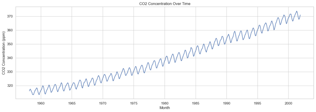
As shown in the chart above, the CO2 concentration in parts per million (ppm) has continuously increased from 1958 to 2001.
Step 3: Identify Model Order
In ARIMA (AutoRegressive Integrated Moving Average) modeling, the model order is represented as (p, d, q), where:
- p (AutoRegressive order): This parameter represents the number of lag observations (time steps from previous periods) included in the model. It reflects the effect of past values on the current value. For example, if p is set to 2, the current value will be influenced by the two immediately preceding time steps.
- d (Integration order): This parameter represents the number of differences needed to make the time series data stationary. Stationarity is crucial in time series analysis, and ‘d’ quantifies the number of times differencing is required to achieve stationarity. If d is 0, the data is already stationary. If it’s 1, the first difference is taken, and if it’s 2, a second difference is applied, and so on.
- q (Moving Average order): This parameter represents the number of lagged forecast errors included in the model. It captures the effect of past forecast errors on the current value. A higher q value means a more extensive consideration of past errors in the model.
When seeking to fit time series data using a seasonal ARIMA model, our initial objective is to discover the optimal values for the ARIMA(p, d, q)(P, D, Q) parameters that maximize a chosen evaluation metric. The approach involves employing a “grid search” method to systematically explore various parameter combinations. For each parameter combination, we create a new seasonal ARIMA model using the SARIMAX() function from the statsmodels module and evaluate its overall performance. After exploring the full spectrum of parameters, the optimal parameter set will be the one that produces the best results according to our chosen evaluation criteria.
############################################
# STEP 3: IDENTIFY MODEL ORDER
############################################

# Define the range of values for p, d, and q parameters between 0 and 2
p = d = q = range(0, 2)

# Generate all possible combinations of p, d, and q triplets.
pdq = list(itertools.product(p, d, q))

# Generate all possible combinations of seasonal p, d, and q triplets with a seasonality of 12.
seasonal_pdq = [(x[0], x[1], x[2], 12) for x in list(itertools.product(p, d, q))]


warnings.filterwarnings("ignore") # specify to ignore warning messages

for param in pdq:
    for param_seasonal in seasonal_pdq:
        try:
            mod = sm.tsa.statespace.SARIMAX(y,
                                            order=param,
                                            seasonal_order=param_seasonal,
                                            enforce_stationarity=False,
                                            enforce_invertibility=False)

            results = mod.fit()

            print('ARIMA{}x{}12 - AIC:{}'.format(param, param_seasonal, results.aic))
        except:
            continue

----------------- OUTPUT -----------------------
ARIMA(1, 1, 1)x(1, 1, 1, 12)12 - AIC:216.3543555875499
------------------------------------------------
We compare statistical models with different parameters by assessing their goodness of fit and predictive performance. We employ the Akaike Information Criterion (AIC) to measure this, a value readily available when fitting ARIMA models using statsmodels. The AIC balances model fit and complexity. It assigns higher AIC scores to models that fit data well but use more features. Our aim is to identify the model with the lowest AIC value.
The code snippet above tests parameter combinations using the SARIMAX function, specifying the (p, d, q) and (P, D, Q, S) parameters for the Seasonal ARIMA model. After each model fit, the code displays its AIC score.
The optimal model, SARIMAX(1, 1, 1)x(1, 1, 1, 12), has the lowest AIC value of 216.35, making it our preferred choice.
Step 4: Fitting Model
Having conducted a grid search, we’ve pinpointed the parameter set for the best-fitting time series model. Now, let’s delve deeper into this specific model by initializing a new SARIMAX model with the optimal parameter values:
############################################
# STEP 4: FITTING MODEL
############################################

mod = sm.tsa.statespace.SARIMAX(y,
                                order=(1, 1, 1),
                                seasonal_order=(1, 1, 1, 12),
                                enforce_stationarity=False,
                                enforce_invertibility=False)

results = mod.fit()

print(results.summary().tables[1])
----------------- OUTPUT -----------------------
==============================================================================
                 coef    std err          z      P>|z|      [0.025      0.975]
------------------------------------------------------------------------------
ar.L1          0.1297      0.122      1.059      0.290      -0.110       0.370
ma.L1         -0.4792      0.111     -4.333      0.000      -0.696      -0.262
ar.S.L12       0.0014      0.002      0.926      0.354      -0.002       0.004
ma.S.L12      -0.8605      0.027    -31.682      0.000      -0.914      -0.807
sigma2         0.0860      0.006     15.403      0.000       0.075       0.097
==============================================================================
------------------------------------------------
The summary attribute that results from the output of SARIMAX returns a significant amount of information.
The p-values assess the statistical significance of the coefficients:
- The p-value for
ar.L1is approximately 0.290, indicating that it’s not statistically significant at a typical significance level (e.g., 0.05). It suggests that the autoregressive termar.L1may not be statistically significant. - The p-value for
ma.L1is approximately 0.000, indicating high statistical significance. - The p-value for
ar.S.L12is approximately 0.354, suggesting that it’s not statistically significant. - The p-value for
ma.S.L12is approximately 0.000, indicating high statistical significance. - The p-value for
sigma2is approximately 0.000, indicating that the error variance term is statistically significant.
The significance of p-values varies by field and analysis context. ar.L1 and ar.S.L12 are not statistically significant. When these coefficients are not statistically significant, it means that including these terms in your model doesn’t significantly improve its ability to fit the data. In this case, it is reasonable to retain all of them in the model.
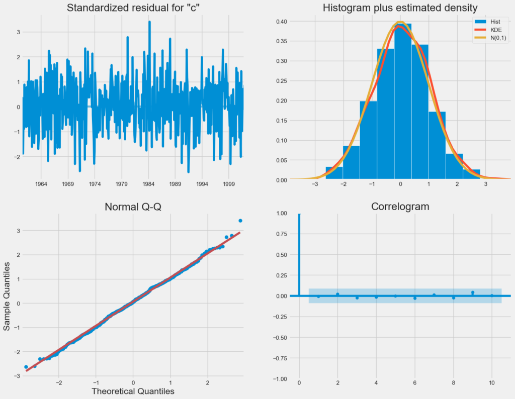
When working with seasonal ARIMA models or any other models, it’s crucial to conduct model diagnostics to verify the model’s underlying assumptions remain valid. Utilizing the plot_diagnostics function, we can efficiently generate diagnostic visualizations and scrutinize the model for any unexpected patterns or irregularities.
results.plot_diagnostics(figsize=(15, 12))
plt.show()
Observations:
- The top-right plot reveals that the red KDE line closely aligns with the N(0,1) line, indicating that the residuals exhibit a normal distribution (N(0,1) represents a standard normal distribution with mean 0 and standard deviation 1).
- In the bottom-left qq-plot, the ordered residuals (blue dots) closely follow a linear trend expected from a standard normal distribution N(0, 1), further supporting the normality of residuals.
- Analyzing the top-left plot, it’s evident that the residuals over time lack significant seasonality and resemble white noise. This observation is corroborated by the autocorrelation plot in the bottom-right, which indicates a low correlation between the time series residuals and their lagged versions.
Based on these observations, we can confidently assert that our model provides a reliable fit, enhancing our ability to comprehend the time series data and make accurate forecasts.
Step 5: Validate Forecasts
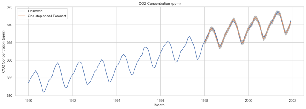
We have developed a time series model that is ready for forecasting. To assess the accuracy of our predictions, we compare them to the actual values in the time series. We use the get_prediction() method to obtain forecasted values and the conf_int() method to access confidence intervals associated with these forecasts.
By specifying dynamic=False, we are ensuring that we create one-step ahead forecasts. In this context, “one step ahead” means that the forecasts at each point in time are generated using the complete historical data up to that point.
We can visualize the actual and forecasted values of the GDP time series to evaluate the model’s performance. We’ve focused on the later part of the time series by selecting a specific date range.
############################################
# STEP 5: VALIDATING FORECAST
############################################

# Generate predictions starting from January 1998
pred = results.get_prediction(start=pd.to_datetime('1998-01-01'), dynamic=False)

# Calculate the confidence interval for the predictions
pred_ci = pred.conf_int()

# Create a DataFrame for the observed data and one-step ahead forecasts
data = pd.DataFrame({'Observed': y['1990':], 'One-step ahead Forecast': pred.predicted_mean})

# Plot the data and forecasts
sns.set(style="whitegrid")
fig, ax = plt.subplots(figsize=(15, 5))
sns.lineplot(data=data, ax=ax, dashes=False)
ax.fill_between(pred_ci.index, pred_ci.iloc[:, 0], pred_ci.iloc[:, 1], color='gray', alpha=0.5)
ax.set(xlabel='Month', ylabel='CO2 Concentration (ppm)')
plt.title('CO2 Concentration (ppm)')
ax.legend()
plt.grid(True)
plt.show()
In general, our forecasts closely match the actual values, indicating a consistent upward trend.
We can assess forecast accuracy by calculating the Mean Squared Error (MSE). The MSE represents the average of the squared differences between our predicted values and the true values. Squaring the differences ensures that both positive and negative discrepancies contribute to the overall measure.
y_forecasted = pred.predicted_mean
y_truth = y['1998-01-01':]

# Compute the mean square error
mse = ((y_forecasted - y_truth) ** 2).mean()
print('The Mean Squared Error of our forecasts is {}'.format(round(mse, 2)))
----------------- OUTPUT -----------------------
The Mean Squared Error of our forecasts is 0.07
------------------------------------------------
The Mean Squared Error (MSE) for our one-step ahead forecasts is remarkably low at 0.07 approaching 0. An MSE of 0 would indicate that the estimator predicts parameter observations with absolute precision, an ideal but usually unattainable scenario.
Step 6: Forecasting
The final step is to project future values and gain insights into future trends. Using the get_forecast() method of our time series object, we can compute forecasted values for a specified number of steps ahead, which is particularly useful for planning and decision-making.
To provide a comprehensive view of the forecasted values, we also compute confidence intervals for these forecasts. This helps us assess the range within which future values are likely to fall, providing a measure of prediction uncertainty.
Here’s how to generate the forecasts and confidence intervals:
############################################
# STEP 6: PRODUCING FORECAST
############################################

# Get forecast 500 steps ahead in future
pred_uc = results.get_forecast(steps=300)

# Get confidence intervals of forecasts
pred_ci = pred_uc.conf_int()
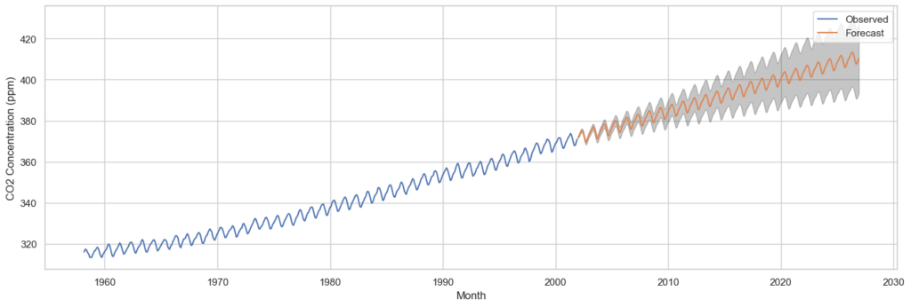
With the forecasted values and their associated confidence intervals in hand, we can visualize the time series along with the forecasts and prediction uncertainty. This graphical representation enhances our understanding of future CO2 levels and allows for informed decision-making.
# Plot using Seaborn
plt.figure(figsize=(15, 5))
ax = sns.lineplot(x=y.index, y=y, label='Observed')
sns.lineplot(x=pred_uc.predicted_mean.index, y=pred_uc.predicted_mean, ax=ax, label='Forecast')
ax.fill_between(pred_ci.index, pred_ci.iloc[:, 0], pred_ci.iloc[:, 1], color='k', alpha=0.25)
ax.set(xlabel='Date', ylabel='CO2 Levels')

plt.legend()
plt.show()
As illustrated in the chart above, the projected CO2 concentration (in parts per million, ppm) is anticipated to reach approximately 410 by 2027, marking a substantial increase from its level of less than 320 in 1958.
Conclusion
ARIMA modeling provides valuable insights and forecasts, enabling us to understand and anticipate the behavior of complex time series data, such as atmospheric CO2 concentrations. By following these steps, we can unlock the potential of ARIMA for various applications, from climate research to financial forecasting and beyond.
References
- Hyndman, R. J., & Athanasopoulos, G.(2018). ARIMA Models. In Forecasting: Principles and Practice. Retrieved from https://otexts.com/fpp2/arima.html
- DigitalOcean. (2017). A Guide to Time Series Forecasting with ARIMA in Python 3. In DigitalOcean Community. Retrieved from https://www.digitalocean.com/community/tutorials/a-guide-to-time-series-forecasting-with-arima-in-python-3#step-6-validating-forecasts