Regression is a predictive modeling technique used when we want to understand the relationship between one or more independent variables and a dependent variable, typically for making numerical predictions. In other words, regression allows us to estimate or forecast a continuous outcome, making it an essential tool for tasks like house price prediction, stock market analysis, and more. By analyzing and learning from historical data, regression models provide valuable insights and enable us to make data-driven decisions.

In this post, I’ll delve into model representation, evaluation metrics, and the concept of regularized regression. I will also explore the essential technique of Cross-Validation. To apply these principles in the blog, I will use Ridge and Lasso regression to predict housing prices in California.

---

1.0 Understanding Regression

1.1 Model Representation

The model representation in linear regression is the mathematical expression that describes the relationship between the dependent variable (the target) and one or more independent variables (features or predictors). It is the core equation that forms the basis of a linear regression model. The general form of the model representation in simple linear regression is as follows:

• Formula: Y = b0 + b1*X + ε

Where:

• Y: The dependent variable (the target you want to predict).
• X: The independent variable (one or more features).
• b0: Intercept (the value of Y when X is 0).
• b1: Coefficient (slope) that represents how much Y changes with a one-unit change in X.
• ε: Residuals (error terms), representing the difference between the predicted and actual Y values.

In the case of multiple linear regression, where there is more than one independent variable, the model representation extends to include all the predictor variables:

• Formula: Y = b0 + b1*X1 + b2*X2 + ... + bn*Xn + ε

Where:

• Y: Remains the dependent variable (the target).
• X1, X2, ..., Xn: Are the independent variables (features or predictors).
• b0, b1, b2, ..., bn: Are the coefficients associated with each independent variable.
• ε: Represents the error term or residuals.

1.2 Evaluation Metrics

Measuring the performance of your models is a critical step. After all, knowing how well the model performs is essential for making informed decisions and improvements. Below, I’ll delve into key evaluation metrics such as R-squared, Mean Squared Error (MSE), and Root Mean Squared Error (RMSE).

1.2.1 R-Squared

The default evaluation metric for linear regression is R-squared. R-squared measures how well the independent variables explain the variation in the dependent variable. It ranges from 0 to 1, where higher values indicate a better fit.

• Formula: R^2 = 1 - (SSR/SST)

Where:

• SSR: Sum of squared residuals (same as MSE)
• SST: Total sum of squares, which measures the total variation in the dependent variable.

The charts below visualize a high R-squared and a low R-squared.

1.2.2 Mean Squared Error (MSE)

MSE calculates the average of the squared differences between the predicted values and the actual values. It emphasizes larger errors more than MAE.

• Formula: MSE = (1/n) * Σ (Y - Ŷ)^2
• Where:
  • Y: Actual values
  • Ŷ: Predicted values
  • n: Number of data points

Lower MSE values indicate that the model’s predictions are closer to the actual values. However, there is no universal threshold for a “good” MSE because the interpretation depends on the scale of the target variable. It’s context-dependent.

1.2.3 Root Mean Squared Error (RMSE)

RMSE is the square root of the MSE and provides an interpretable measure of the model’s error in the same units as the target variable.

• Formula: RMSE = √(MSE)

Just like MSE, lower RMSE values are generally better. RMSE provides a more interpretable measure of error because it’s in the same units as the target variable.

1.3 Regularized Regression

Ridge and Lasso regression are two commonly used techniques in machine learning for linear regression problems. They are both used to improve the stability and generalizability of linear regression models by addressing issues like multicollinearity* and overfitting.

*Multicollinearity occurs when two or more independent variables are highly correlated. Multicollinearity can be problematic for several reasons:

• Interpretability: It makes it challenging to understand the individual impact of each feature on the prediction because their effects are entangled.
• Stability: It can lead to unstable and unreliable coefficient estimates in regression models.

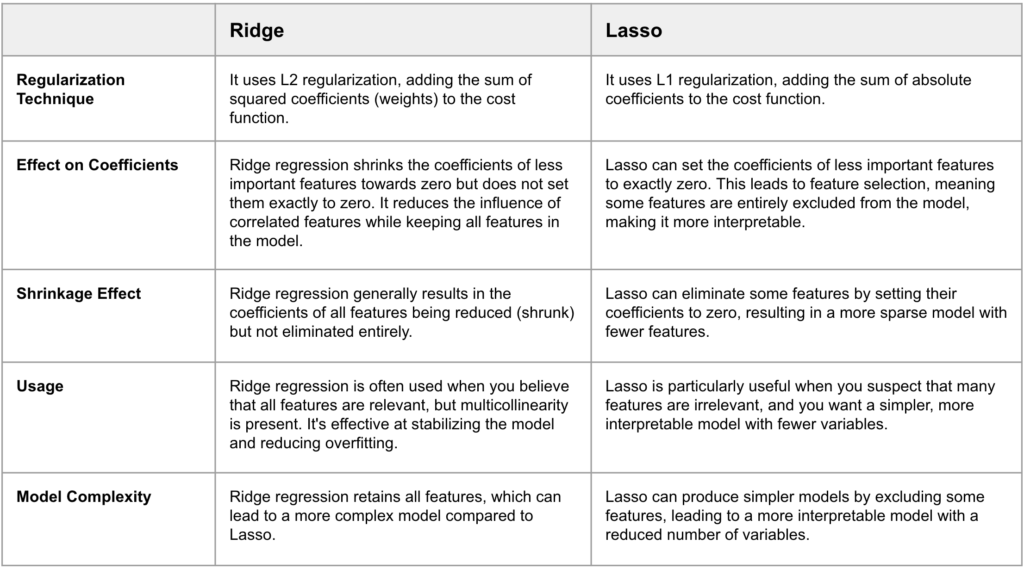
In summary, Ridge regression and Lasso are both regularization techniques used to improve linear regression models. Ridge focuses on reducing the influence of correlated features while keeping all features, while Lasso can eliminate some features entirely, leading to a sparser and simpler model. The choice between the two depends on the nature of the dataset and the specific goals of the analysis.

---

2.0 Cross Validation

Cross-validation is a widely used technique in machine learning for assessing the performance of a predictive model. It is a form of cross-validation that helps in estimating how well a model is likely to perform on an independent dataset. Below is an example of 5-fold cross-validation:

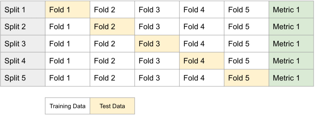
• Data Splitting: The dataset is divided into five approximately equal-sized subsets or folds.
• Training and Testing: The model is then trained and evaluated five times. In each interaction, four of the folds are used for training, and the remaining one is used for testing.
• Evaluation: During each iteration, the model’s performance is evaluated using a chosen evaluation metric (e.g., accuracy, mean squared error, or another relevant metric).
• Average Performance: After all five iterations are complete, the performance scores are averaged. This average provides a more reliable estimate of the model’s performance compared to evaluating it on a single fixed test set.

---

3.0 Regression with Python

In the Python code that follows, we’ll put regression principles into action. We’ll kick off by loading a dataset and then dive into exploratory data analysis (EDA). Afterward, we’ll pinpoint the optimal alpha score and construct both Ridge and Lasso Regression models. Finally, we’ll evaluate the models’ performance.

3.1 Load Data

The dataset that we will use is the “California Housing Prices” which was derived from the 1990 U.S. census. It contains data related to housing prices in various districts in California. Each row in the dataset represents one district, and the columns provide information about features like population, median income, and housing prices.

############################################
# STEP 1: LOAD DATASET
############################################

from sklearn.datasets import fetch_california_housing

# Load the California Housing dataset
data = fetch_california_housing()

# Convert the dataset into a Pandas DataFrame for easier exploration
df = pd.DataFrame(np.c_[data.data, data.target], columns= list(data.feature_names) + ['target'])

# Print Column Names
print(df.columns)

----------------- OUTPUT -----------------------
Index(['MedInc', 'HouseAge', 'AveRooms', 'AveBedrms', 'Population', 'AveOccup',
       'Latitude', 'Longitude', 'target'],
      dtype='object')
------------------------------------------------

Here’s a description of each of the columns in the dataset:

1. MedInc (Median Income): The median income of households in a district.
2. HouseAge (Housing Age): The median age of houses in the district.
3. AveRooms (Average Rooms): The average number of rooms per dwelling in the district.
4. AveBedrms (Average Bedrooms): The average number of bedrooms per dwelling.
5. Population: The total population in the district.
6. AveOccup (Average Occupancy): The average occupancy of households in the district.
7. Latitude: The latitude of the district’s geographical location.
8. Longitude: The longitude of the district’s geographical location.
9. Target: The median value of the home, expressed in hundreds of thousands of dollars ($100,000).

3.2 Explore Dataset

The second step is exploratory data analysis (EDA) on the dataset.

############################################
# STEP 2: EXPLORE DATASET
############################################

# Check for missing values in the dataset
print("Missing values:")
print(df.isnull().sum())
----------------- OUTPUT -----------------------
MedInc        0
HouseAge      0
AveRooms      0
AveBedrms     0
Population    0
AveOccup      0
Latitude      0
Longitude     0
target        0
dtype: int64
------------------------------------------------

# Check for the unique number of values
print("The unique number of data values are")
df.nunique()

----------------- OUTPUT -----------------------
MedInc        12928
HouseAge         52
AveRooms      19392
AveBedrms     14233
Population     3888
AveOccup      18841
Latitude        862
Longitude       844
target         3842
dtype: int64
------------------------------------------------

As seen in the Python code above, there are no missing values in the dataset, and the number of distinct values varies across different columns.

# Visualize the distribution of the target variable
plt.figure(figsize=(15, 5))
sns.histplot(df['target'], bins=30, kde=True)
plt.title("Distribution of Median House Values")
plt.xlabel("Median House Value (in thousands of USD)")
plt.show()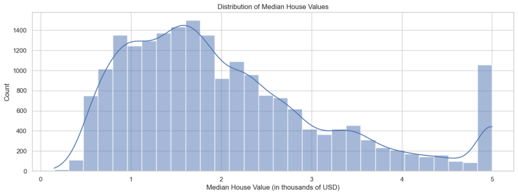

As seen in the chart above, most of the “Median House Values” fall within the range of 1 (representing $100,000) to 2 (representing $200,000). The values start declining after reaching 2, but there is another increase just before reaching 5.

# Visualize correlations between features
correlation_matrix = df.corr()
plt.figure(figsize=(15, 5))
sns.heatmap(correlation_matrix, annot=True, cmap="coolwarm")
plt.title("Feature Correlation Heatmap")
plt.show()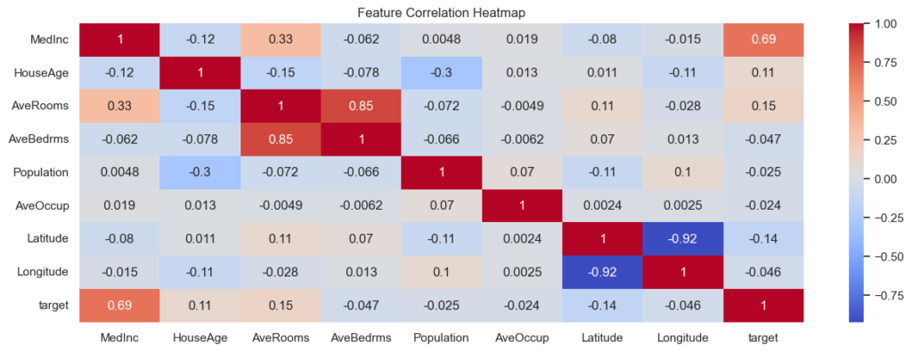

As seen in the Correlation Heatmap, “MedInc” and “Target” have the highest positive correlation of approximately 0.69. It suggests that higher median income is strongly associated with higher median house values.

plt.figure(figsize=(12, 8))
plt.scatter(df['Longitude'], df['Latitude'], c=df['target'], cmap='coolwarm', s=20)
plt.colorbar().set_label('Median House Value (in thousands of USD)')
plt.title('Median House Value by Geographical Coordinates')
plt.xlabel('Longitude')
plt.ylabel('Latitude')
plt.grid(True)
plt.show()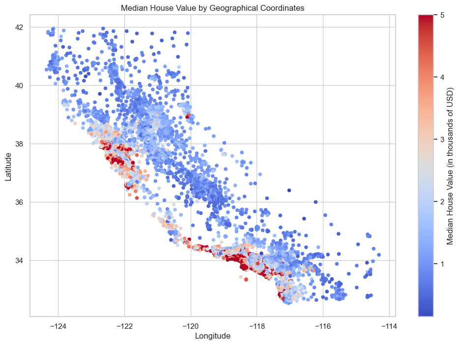

As observed in the visualization above, the regions with the highest house prices correspond to San Francisco, Los Angeles, and San Diego.

3.3 Identify Optimal Alpha Score

After exploring the dataset, it is now time to build Ridge and Lasso regression models. As mentioned earlier, these regularization techniques are essential for improving the robustness of your models by preventing overfitting and making your predictions more stable.

As seen in the Python code below, we first identify the optimal alpha for Ridge and Lasso. The goal is to determine the level of regularization that optimizes the model’s fit to the data.

A range of alpha values (regularization strength) is specified in the alphas list. These alpha values control the amount of regularization applied to the model. A smaller alpha value implies less regularization, while a larger alpha value implies more regularization.

A loop iterates over the alpha values, and for each alpha, a regression model is created with that specific regularization strength. After evaluating all alpha values, the code finds the highest R-squared score and its corresponding alpha.

############################################
# STEP 3: OPTIMAL RIDGE ALPHA
############################################
from sklearn.linear_model import Ridge

X = data.data
y = data.target

# Define the alpha values
alphas = [0.1, 1.0, 10.0, 100.0, 1000.0, 10000.0]

# Initialize a list to store R-squared scores
ridge_scores = []

# Create Ridge regression models for different alpha values and calculate R-squared
for alpha in alphas:
    ridge = Ridge(alpha=alpha)
    ridge.fit(X, y)
    score = ridge.score(X, y)
    ridge_scores.append(score)

# Find the highest R-squared score and its corresponding alpha
max_score = max(ridge_scores)
best_alpha = alphas[ridge_scores.index(max_score)]

print("Highest R-squared Score:", max_score)
print("Corresponding Alpha Value:", best_alpha)
----------------- OUTPUT -----------------------
Highest R-squared Score: 0.6062326849340285
Corresponding Alpha Value: 0.1
------------------------------------------------

############################################
# STEP 3: OPTIMAL LASSO ALPHA
############################################

from sklearn.linear_model import Lasso
X = data.data
y = data.target

# Define the alpha values
alphas = [0.1, 1.0, 10.0, 100.0, 1000.0, 10000.0]

# Initialize a list to store R-squared scores
lasso_scores = []

# Create Lasso regression models for different alpha values and calculate R-squared
for alpha in alphas:
    lasso = Lasso(alpha=alpha)
    lasso.fit(X, y)
    score = lasso.score(X, y)
    lasso_scores.append(score)

# Find the highest R-squared score and its corresponding alpha
max_score = max(lasso_scores)
best_alpha = alphas[lasso_scores.index(max_score)]

print("Highest R-squared Score:", max_score)
print("Corresponding Alpha Value:", best_alpha)
----------------- OUTPUT -----------------------
Highest R-squared Score: 0.5452665703368436
Corresponding Alpha Value: 0.1
------------------------------------------------

The two outputs display the highest R-squared score by Ridge and Lasso and the optimal alpha value. As seen, Ridge has the highest R-squared score, and the optimal alpha value is 0.1 for both of them.

# Ridge
----------------- OUTPUT -----------------------
Highest R-squared Score: 0.6062326849340285
Corresponding Alpha Value: 0.1
------------------------------------------------

# Lasso
----------------- OUTPUT -----------------------
Highest R-squared Score: 0.5452665703368436
Corresponding Alpha Value: 0.1
------------------------------------------------

3.4 Build Ridge and Lasso Regression Model

After identifying the optimal alpha score for Ridge and Lasso regression models, the next step is to create the regression models with the score.

The model’s performance is evaluated using 5-fold cross-validation. This means the dataset is split into 5 subsets (folds). The model is trained on 4 of these folds and tested on the remaining one in each iteration. This process is repeated 5 times to obtain a set of R-squared scores. After cross-validation, the model is fitted to the entire dataset (X, y). This step trains the model on the complete dataset.

Then the code calculates the R-squared score on the entire dataset to assess how well the model fits the data as a whole. Finally, the code prints the R-squared scores obtained from cross-validation, providing insights into how the model performs on different subsets of the data. It also displays the overall R-squared score, indicating the model’s fit to the entire dataset.

############################################
# STEP 4: BUILD RIDGE REGRESSION MODEL
############################################
from sklearn.model_selection import cross_val_score

# Create a Ridge regression model
ridge_model = Ridge(alpha=0.1) #Optimal Alpha Score

# Perform 5-fold cross-validation and get the R-squared scores
scores = cross_val_score(ridge_model, X, y, cv=5, scoring='r2')

# Fit the model to the entire dataset
ridge_model.fit(X, y)

# Calculate the R-squared score on the entire dataset
overall_r2 = ridge_model.score(X, y)

# Print cross-validation scores and overall R-squared score
print("Cross-Validation R-squared Scores:", scores)
print("Overall R-squared Score:", overall_r2)

----------------- OUTPUT -----------------------
Cross-Validation R-squared Scores: [0.54867555 0.46820356 0.55078438 0.5369819  0.66051573]
Overall R-squared Score: 0.6062326849340285
------------------------------------------------

############################################
# STEP 4: BUILD LASSO REGRESSION MODEL
############################################

# Create a Lasso regression model with the best alpha
lasso_model = Lasso(alpha=0.1) #Optimal Alpha Score

# Perform 5-fold cross-validation and get the R-squared scores
scores = cross_val_score(lasso_model, X, y, cv=5, scoring='r2')

# Fit the model to the entire dataset
lasso_model.fit(X, y)

# Calculate the R-squared score on the entire dataset
overall_r2 = lasso_model.score(X, y)

# Print cross-validation scores and overall R-squared score
print("Cross-Validation R-squared Scores:", scores)
print("Overall R-squared Score:", overall_r2)
----------------- OUTPUT -----------------------
Cross-Validation R-squared Scores: [0.51250667 0.42928553 0.51135698 0.38784761 0.51998859]
Overall R-squared Score: 0.5452665703368436
------------------------------------------------

3.5 Model Evaluation

In our pursuit of optimizing the model’s performance, we experimented with both Ridge and Lasso regression. As seen below, the Ridge model yielded an R-squared score of 0.6062 indicating a reasonably good fit to the data. On the other hand, Lasso regression resulted in an R-squared score of 0.5452 slightly lower than Ridge.

From these results, it appears that the Ridge model performed better in this particular scenario, given its higher R-squared score. This suggests that the level of regularization applied by Ridge was more appropriate for the dataset, as it produced a more accurate fit.

# Ridge
----------------- OUTPUT -----------------------
Cross-Validation R-squared Scores: [0.54867555 0.46820356 0.55078438 0.5369819  0.66051573]
Overall R-squared Score: 0.6062326849340285
------------------------------------------------

# Lasso
----------------- OUTPUT -----------------------
Cross-Validation R-squared Scores: [0.51250667 0.42928553 0.51135698 0.38784761 0.51998859]
Overall R-squared Score: 0.5452665703368436
------------------------------------------------

4.0 Conclusion

Throughout this post, we’ve explored key concepts in regression, including model representation, evaluation metrics, and regularized regression. We’ve also touched on the essential technique of cross-validation. Applying these principles to a real-world scenario, we used Ridge and Lasso regression to predict housing prices in California.

We began by loading the “California Housing Prices” dataset and delved into exploratory data analysis, gaining insights into the data’s features and correlations. Next, we determined the optimal alpha scores for Ridge and Lasso to control the level of regularization. After identifying the optimal alpha values, we built Ridge and Lasso regression models, evaluated their performance using cross-validation, and assessed their overall fit to the dataset. Ridge demonstrated a higher R-squared score, indicating a better fit to the data.

In summary, regression techniques like Ridge and Lasso provide powerful tools for predictive modeling and understanding complex relationships in real-world datasets.