Support Vector Machines (SVM) is a popular machine learning technique used for classification tasks. SVMs excel at finding the best boundary to separate different classes of data by maximizing the margin between them.
Simplified Explanation
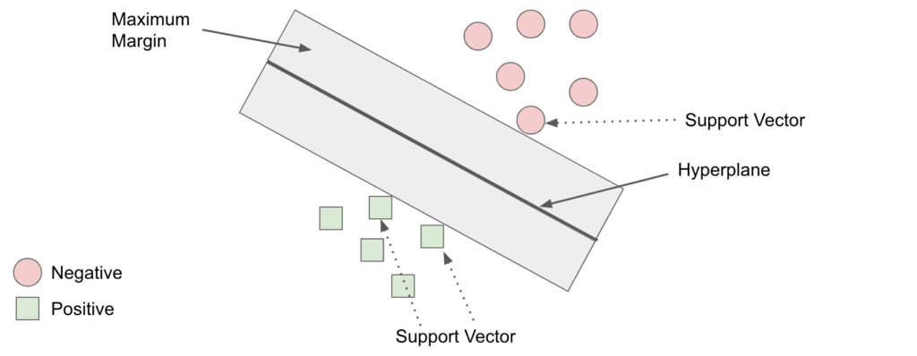
SVM selects the best line to separate different groups of data by making sure it is as far away as possible from the groups. This makes it a “maximum margin classifier”.
Now, imagine some data points are like “troublemakers” because they are very close to this line, and deciding which group they belong to is tough. We call these troublemakers “support vectors”.
Here’s the key: Only these troublemaker support vectors affect where the line goes. If we move a troublemaker, the line moves with it. But the other data points don’t matter much. So, support vectors are the real decision-makers when it comes to drawing the line.

In this post…
We’re going to create a classification Support Vector Machine using scikit-learn. We have a training dataset with a mix of continuous and categorical data sourced from the UCI Machine Learning Repository. Our goal is to use this data to predict if a person will default on their credit card or not.
Step 1: Load Libraries & Import Data
This code sets up a classification task to predict credit card default. It loads required libraries, imports the dataset, renames a column, and drops an unnecessary one.
import pandas as pd
import numpy as np
import matplotlib.pyplot as plt
import matplotlib.colors as colors
from sklearn.utils import resample
from sklearn.model_selection import train_test_split
from sklearn.preprocessing import scale
from sklearn.svm import SVC
from sklearn.model_selection import GridSearchCV
from sklearn.metrics import confusion_matrix, ConfusionMatrixDisplay
from sklearn.decomposition import PCA


############################################
# STEP 1: LOAD DATA
############################################

# Load dataset
df = pd.read_csv('UCI_Credit_Card.csv')

# Rename Column Name
df.rename({'default.payment.next.month':'DEFAULT'},axis='columns',inplace=True)

# Drop ID column (not important)
df.drop('ID',axis=1,inplace=True)
Step 2: Missing Data & Downsample
This code examines and cleans a dataset for a credit card default prediction project. It starts by checking data types, unique values, and identifying invalid data. Then, it removes rows with invalid data. Afterwards, it splits the data into two groups: one for credit card defaults and one for non-defaults. Finally, it downsamples both groups to create a balanced dataset for analysis. The final dataset has 2,000 rows, with 1000 rows representing each class (default and no default).
############################################
# STEP 2: MISSING DATA
############################################

# Check data types of columns in the DataFrame
df.dtypes
----------------- OUTPUT -----------------------
LIMIT_BAL    float64 # Credit Limit
SEX            int64 # Gender
EDUCATION      int64 # Level of Education
MARRIAGE       int64 # Marital Status
AGE            int64 # Age
PAY_0          int64 # When the bills were payed
PAY_2          int64 # When the bills were payed
PAY_3          int64 # When the bills were payed
PAY_4          int64 # When the bills were payed
PAY_5          int64 # When the bills were payed
PAY_6          int64 # When the bills were payed
BILL_AMT1    float64 # What the last bill was
BILL_AMT2    float64 # What the last bill was
BILL_AMT3    float64 # What the last bill was
BILL_AMT4    float64 # What the last bill was
BILL_AMT5    float64 # What the last bill was
BILL_AMT6    float64 # What the last bill was
PAY_AMT1     float64 # How much the last payment was
PAY_AMT2     float64 # How much the last payment was
PAY_AMT3     float64 # How much the last payment was
PAY_AMT4     float64 # How much the last payment was
PAY_AMT5     float64 # How much the last payment was
PAY_AMT6     float64 # How much the last payment was
DEFAULT        int64
------------------------------------------------

# Check unique values in the 'SEX', 'EDUCATION', and 'MARRIAGE' columns
df['SEX'].unique()
df['EDUCATION'].unique()
df['MARRIAGE'].unique()

# Count and document the number of rows with 'EDUCATION' or 'MARRIAGE' values equal to 0
len(df.loc[(df['EDUCATION'] == 0) | (df['MARRIAGE'] == 0)]) # 68

# Total number of rows in the DataFrame
len(df) # 30,000

# Create a new DataFrame with rows that have valid 'EDUCATION' and 'MARRIAGE' values
df_no_missing = df.loc[(df['EDUCATION'] != 0) & (df['MARRIAGE'] != 0)]

# Number of rows in the cleaned DataFrame
len(df_no_missing) # 29,932

# Split the data into two DataFrames: one with no defaults and one with defaults
df_no_default = df_no_missing[df_no_missing['DEFAULT'] == 0]
df_default = df_no_missing[df_no_missing['DEFAULT'] == 1]

# Downsample the 'no default' and 'default' DataFrames to 1000 rows each
df_no_default_downsampled = resample(df_no_default, replace=False,n_samples=1000,random_state=42)
df_default_downsampled = resample(df_default, replace=False,n_samples=1000,random_state=42)

# Combine the downsampled DataFrames to create a balanced dataset
df_downsample = pd.concat([df_no_default_downsampled, df_default_downsampled])

# Number of rows in the downsampled DataFrame
len(df_downsample) # 2000
Step 3: Exploratory Data Analysis
Exploratory Data Analysis (EDA) is a fundamental phase in the data analysis process that involves examining and understanding the structure, characteristics, and patterns within a dataset. In this section, we will conduct EDA on the UCI Credit Card Default dataset to gain a comprehensive understanding of the data and the relationships between its variables.
############################################
# STEP 3: EDA
############################################

# Age distribution for default and non-default customers

# Create age ranges
age_ranges = [20,25,30,35,40,45,50,55,60,65,70]

# Create age bins
df_downsample['AgeRange'] = pd.cut(df_downsample['AGE'], bins=age_ranges)

# Calculate the percentage of default and non-default cases in each age range
age_percentages = df_downsample.groupby(['AgeRange', 'DEFAULT']).size().unstack(fill_value=0).apply(lambda x: x / x.sum() * 100, axis=1)

# Plot the percentages
plt.figure(figsize=(15, 5))
age_percentages.plot(kind='bar', stacked=True, color=['skyblue', 'salmon'])
plt.title('Percentage of Default and Non-default by Age Range')
plt.xlabel('Age Range')
plt.ylabel('Percentage')
plt.xticks(rotation=45)
plt.legend(['Non-default', 'Default'])
plt.show()
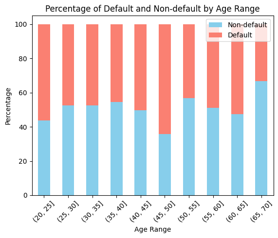
As seen in the stacked bar chart above, the age group characterized by the highest default percentage falls within the range of 45 to 50 years, closely followed by individuals aged between 20 and 25 years. In contrast, the age group exhibiting the lowest default rate consists of individuals between 65 and 70 years of age.
# Credit limit distribution for default and non-default customers

# Create credit limit ranges
credit_limit_ranges = [0, 20000, 40000, 60000, 80000, 100000, 150000, 200000, 300000, 500000, float('inf')]

# Create credit limit bins
df_downsample['CreditLimitRange'] = pd.cut(df_downsample['LIMIT_BAL'], bins=credit_limit_ranges)

# Calculate the percentage of default and non-default cases in each range
credit_limit_percentages = df_downsample.groupby(['CreditLimitRange', 'DEFAULT']).size().unstack(fill_value=0).apply(lambda x: x / x.sum() * 100, axis=1)

# Plot the percentages
plt.figure(figsize=(15, 5))
credit_limit_percentages.plot(kind='bar', stacked=True, color=['skyblue', 'salmon'])
plt.title('Percentage of Default and Non-default by Credit Limit')
plt.xlabel('Credit Limit Range')
plt.ylabel('Percentage')
plt.xticks(rotation=45)
plt.legend(['Non-default', 'Default'])
plt.show()
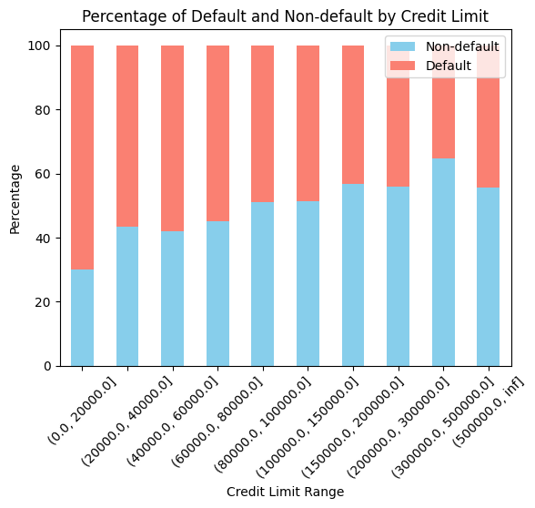
Evident from the chart above is the inverse relationship between credit limit ranges and default percentages: as the credit limit range increases, the default percentage decreases. The inverse relationship between credit limit range and default percentages can be explained by factors such as creditworthiness, risk assessment, and the ability to manage debt. Customers with higher credit limits typically have better financial stability and lower default rates.
Step 4: Formatting Data
Data preprocessing is an essential preliminary step in the data analysis pipeline. It involves preparing the dataset for further analysis and modeling by addressing issues related to the structure and format of the data. In this section, we focus on transforming the features and target variable to make them suitable for machine learning.
- Features: The dataset is divided into features represented by the variable ‘X.’ This step involves excluding the ‘DEFAULT’ column, which is our target variable, from the feature set.
- Target: The target variable, ‘y,’ is extracted and isolated for classification tasks. In this context, ‘DEFAULT’ signifies whether a credit card holder defaults or not.
- One-Hot Encoding: Categorical variables such as ‘SEX,’ ‘EDUCATION,’ ‘MARRIAGE,’ and payment statuses (‘PAY_0’ to ‘PAY_6’) are subjected to one-hot encoding. This process converts categorical attributes into a numerical format, making them amenable to machine learning algorithms. It ensures that categorical features can be utilized effectively in predictive models.
############################################
# STEP 4: FORMATTING DATA
############################################

# Features
X = df_downsample.drop('DEFAULT',axis=1).copy()

# Target
y = df_downsample['DEFAULT'].copy()

# One-Hot Encoding
X_encoded = pd.get_dummies(X,columns=['SEX',
                                      'EDUCATION',
                                      'MARRIAGE',
                                      'PAY_0',
                                      'PAY_2',
                                      'PAY_3',
                                      'PAY_4',
                                      'PAY_5',
                                      'PAY_6'])
Step 5: Centering & Scaling
In a machine learning process, it is often essential to standardize or scale the features of the dataset to ensure that they contribute equally to model training and evaluation. This step is particularly crucial when working with algorithms that are sensitive to the scale of the input data. In this section, we focus on centering and scaling the dataset, a fundamental practice for data preparation.
The primary objectives of centering and scaling are as follows:
- Data Splitting: The dataset is divided into training and testing subsets using the
train_test_splitfunction. This division is vital for model training and evaluation, ensuring that models are tested on unseen data. - Feature Scaling: Each feature is independently scaled to have a mean of zero and a standard deviation of one. This process, often referred to as Z-score normalization, is achieved through the
scalefunction. Feature scaling makes features more comparable and prevents attributes with larger scales from dominating the modeling process.
By centering and scaling the data, we ensure that the model can effectively work with features of varying magnitudes, ultimately improving its performance and interpretability. This practice is particularly crucial in cases where different features have substantially different scales or units of measurement.
############################################
# STEP 5: CENTERING AND SCALING
############################################

# Split the dataset into training and testing sets using train_test_split
X_train, X_test, y_train, y_test = train_test_split(X_encoded, y, random_state=42)

# Scale the features in the training set
X_train_scaled = scale(X_train)

# Scale the features in the testing set
X_test_scaled = scale(X_test)
Step 6: Build Model
The code in this section performs a sequence of steps for training a Support Vector Machine (SVM) classifier and evaluating its performance using a confusion matrix.
Classifier Initialization:
- In the first line, a Support Vector Machine (SVM) classifier is created and assigned to the variable
clf_svm. Therandom_stateparameter is set to 42 to ensure reproducibility. Therandom_stateparameter is used to initialize the internal random number generator of the SVM, which can affect its behavior, especially when there are multiple random elements involved.
Classifier Training:
- The SVM classifier is trained on the scaled training data. Scaled features are important to ensure that features with different scales do not dominate the learning process. The
fitmethod is used to train the classifier on the training data (X_train_scaled) and the corresponding target labels (y_train).
Confusion Matrix Calculation:
- This section calculates the confusion matrix to evaluate the classifier’s performance. A confusion matrix is a table that provides a summary of the classifier’s predictions, showing true positives, true negatives, false positives, and false negatives.
# Create a Support Vector Machine (SVM) classifier with a fixed random state
clf_svm = SVC(random_state=42)

# Train the SVM classifier on the scaled training data
clf_svm.fit(X_train_scaled, y_train)

# Calculate the confusion matrix using the trained SVM model and test data
confusion_matrix = ConfusionMatrixDisplay.from_estimator(clf_svm, X_test_scaled, y_test, display_labels=["Did not default", "Defaulted"])

# Display the confusion matrix with specified value formatting
confusion_matrix.plot(values_format='d')
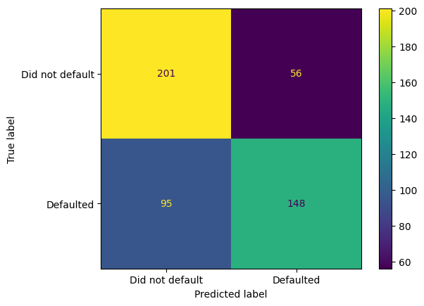
The output of the confusion matrix provides a breakdown of the model’s predictions and their alignment with the actual labels.
As observed, the model accurately predicted that customers did not default on their credit card payments in 201 out of a total of 257 cases (201 correct and 56 incorrect), achieving an accuracy rate of 78.21%. Furthermore, the model correctly identified customers who defaulted in 148 out of 243 cases (148 correct and 95 incorrect), resulting in a true positive rate of 60.90%.
Conclusion
We explored the practical application of Support Vector Machines (SVM) for credit card default prediction. We begin with data preparation, conduct exploratory data analysis (EDA) to gain insights into age and credit limit distributions, format the data, and perform centering and scaling to standardize features. Subsequently, we train an SVM classifier and evaluate its performance using a confusion matrix. The model achieves a 78.21% accuracy in predicting “Did not default” and a 60.90% true positive rate for “Defaulted” cases, demonstrating the value of SVMs in classification tasks and leaving room for potential performance optimization through parameter tuning.
References