This blog post aims to simplify complex financial concepts, including bond valuations, through concise Python code snippets.
We start by clarifying compound interest, showcasing Python’s power to calculate future values and compound interest dynamically. The blog introduces financial functions from numpy_financial, demonstrating their role in solving real-world financial problems.
Moving to bonds, we demystify zero-coupon and coupon bonds with Python, calculating present values for different bond types. We then explore the dynamic relationship between bond prices and yields, illustrating the inverse correlation through Python visualizations.
The blog dives into interest rate sensitivity, using Python to showcase how changing interest rates impact bond prices. We explain the crucial concept of duration and its relationship with bond maturity.
Finally, we delve into convexity, a measure of curvature in the bond’s price-yield relationship, using Python to visualize its relationship with yields.
Time Value of Money
Compound Simple Interest
Calculating compound interest in a bond analysis involves determining how the interest payments on a bond grow over time as they accumulate and are reinvented. Compound interest differs from simple interest, where the interest payments remain constant throughout the bond’s life.
The Python code below calculates the future value of the savings account and the total amount of compound interest earned over a specified period of time.
#########################################################
# COMPOUND INTEREST
#########################################################

# Assign present value, rate and number of periods
pv = 1000
r = 0.03 # 3% interest rate
n = 12 # 12 months

# Calculate the value of the savings account
fv = pv * (1 + r) ** n
print(fv)
----------------- OUTPUT -----------------------
1425.7608868461793
------------------------------------------------

# Calculate the total amount of compound interest earned
compound_interest = fv - pv
print(compound_interest)
----------------- OUTPUT -----------------------
425.76088684617935
------------------------------------------------
This code calculates the future value and compound interest of a savings account with an initial deposit of $1,000, a 3% interest rate, and monthly compounding over 12 months. It outputs the future value, approximately $1,425.76, and the total compound interest earned, approximately $425.76.
Compound Simple Interest with Multiple Cash Flows
When we have multiple cash flows (money transactions) involved, such as investments or loans with deposits or withdrawals at different points in time, we need to use more advanced financial mathematics to calculate the total interest.
The Python code below calculates the future value (fv) of investment and essentially determines how much money will be accumulated after 3 months, considering a 3% monthly interest rate and monthly top-ups.
#########################################################
# COMPOUND INTEREST WITH MULTIPLE CASH FLOWS
#########################################################

import numpy_financial as npf

npf.fv(rate=0.03, # Rate: 3% per period (per month)
       nper=3, # Number of periods: 3 months
       pmt=-100, # Payments: USD -100 top ups at the end of each month
       pv=-1000 # PV: USD -1,000 deposit (pay 1,000 at the beginning)
       )
----------------- OUTPUT -----------------------
1401.817
------------------------------------------------
An initial deposit of $1,000, monthly $100 top-ups, and a 3% interest rate over 3 months would result in a future value of $1,401.
Financial Functions using numpy_financial
number_financial is a Python library that contains functions for financial calculations, such as feature value, present value, interest rate calculations, and more. Below, I will illustrate a few examples.
nper()
The nper() function determines the number of compounding periods required to reach a certain financial goal based on a given interest rate, payment amount, and other financial parameters.
For instance, if we invest $100 per month at 3% compounded monthly. How long time does it take to reach $1,000?
#########################################################
# NPER()
#########################################################

npf.nper(rate=0.03/12, pmt=-100, pv=0, fv=1000)

----------------- OUTPUT -----------------------
9.8893862
------------------------------------------------
As seen above, if we invest $100 per month at 3% compounded monthly, it will take 9.889 months to reach $1,000.
pmt()
The pmt() function determines the payment amount required to grow the present value (PV) to future value (FT).
For instance, if we borrowed $1M at an annual rate of 3% compounded monthly, what monthly payment is required to pay off the loan in 30 years?
#########################################################
# PMT()
#########################################################

npf.pmt(rate=0.03/12, nper=30*12, pv=1000000, fv=0)

----------------- OUTPUT -----------------------
-4216.040337294559
------------------------------------------------
As seen above, to pay off a loan of $1M in 30 years with an annual rate of 3% compounding monthly, the monthly payment would be $4,216.
rate()
The rate() function determines the interest rate required to grow the present value (PV) to future value (FT).
For instance, if we save $1,000 each month, and want to end up with $1M in 30 years, with an interest rate compounded monthly, what rate would be required?
#########################################################
# RATE()
#########################################################

12 * npf.rate(nper=30*12, pmt=-1000, pv=0, fv=1000000)
# Mulitply by 12 to get annual rate required

----------------- OUTPUT -----------------------
0.0597
------------------------------------------------
As seen above, to end up with $1M in 30 years, we would need an annual rate of 5.97%.
pv()
The pv() function determines the prevent (not future) value based on rate, periods, cash flows, and future value.
For instance, how much should we invest now at 3% per year to have $10,000 in 10 years?
#########################################################
# PV()
#########################################################

npf.pv(rate = 0.03, nper=10, pmt=0, fv=10000)

----------------- OUTPUT -----------------------
-7440
------------------------------------------------
We should invest $7,440 per year, at 3% per year, to have $10,000 in 10 years.
Bonds
Bonds are debt securities issued by governments, municipalities, or corporations to raise capital. When an investor purchases a bond, they are essentially lending money to the issuer in exchange for periodic interest payments (coupon payments) and the return of the bond’s face value (principal) at maturity. Bonds are typically considered safer investments than stocks and offer fixed or variable interest rates, making them a source of regular income for investors. The bond’s price and yield can fluctuate in response to changes in interest rates and market conditions, impacting its market value.
Zero-Coupon Bonds
Zero-coupon bonds, often called “zeros,” are a type of bond that doesn’t pay periodic interest (coupon payments) like traditional bonds. Instead, they are issued at a discount to their face value (par value) and pay no interest during their term. Investors buy these bonds at a lower price and receive the face value when the bond matures. The difference between the purchase price and the face value represents the investor’s return, and this is how they earn interest on zero-coupon bonds. They are often used for long-term financial planning and as a way to invest for a future financial goal.
Let’s assume that a zero-coupon bond with a 3-year maturity that yields 3% and has a face value of $100. To determine the present value, we can use the pv() function as previously described:
#########################################################
# ZERO-COUPON BONDS
#########################################################

-npf.pv(rate=0.03, nper=3, pmt=0, fv=100)

----------------- OUTPUT -----------------------
91.51416593531596
------------------------------------------------
As seen above, a zero-coupon bond with a 3-year maturity that yields 3% and has a face value of $100 has a $91.51 present value.
Coupon Bonds
A coupon bond is a type of debt security or financial instrument that pays periodic interest payments (coupons) to the bondholder throughout its term, in addition to returning the bond’s face value (principal) upon maturity.
The primary difference between a coupon bond and a zero-coupon bond is that a coupon bond pays periodic interest (coupons) to the bondholder, along with the return of the face value at maturity, whereas a zero-coupon bond does not pay periodic interest but is sold at a discount, with the bondholder receiving a single lump-sum payment equal to the face value at maturity.
Let’s say that we have a 3-year bond with a 3% annual coupon, face value of $100, and yield of 4%. We can then use the following Python code to calculate the present value.
#########################################################
# COUPON BOND
#########################################################

-npf.pv(rate=0.04, nper=3, pmt=3, fv=100)

----------------- OUTPUT -----------------------
97.22490896677287
------------------------------------------------
Let’s calculate the present value for each of the three years:
- Year 1:
- Initial cash flow: $3 (3% annual coupon of face value)
- Present value: 3/(1+0.04)^1 = 2.8846
- Year 2:
- Initial cash flow: $3 (3% annual coupon of face value)
- Present value: 3/(1+0.04)^2 = 2.7748
- Year 3:
- Initial cash flow: $3 (3% annual coupon of face value)
- Present value: 100/(1+0.04)^3 = 88.5645
Total Present Value = 2.8846 + 2.7758 + 88.5645 = 94.225
So, the present value of the cash flows, broken down by year, is as follows:
- Year 1: $2.8846
- Year 2: $2.7758
- Year 3: $88.5645
The total present value over the three years is $94.225. This means that the combination of payments of $3 in the first two years and the $100 face value in the third year, when discounted at a 4% annual interest rate, is worth about $94.225 in today’s terms.
Bond Prices & Bond Yield
The bond prices are the cost of buying a bond, and bond yield is the return you receive from holding the bond. These two concepts are interconnected, with bond prices and yields often moving in opposite directions: when bond prices go up, yields tend to go down, and vice versa.
The Yield to Maturity (YTM) is a measure of the total return you can expect to earn on a bond if you hold it until it matures, taking into account the bond’s current market price, its face value, the annual interest payments (coupon), and the time left until maturity.
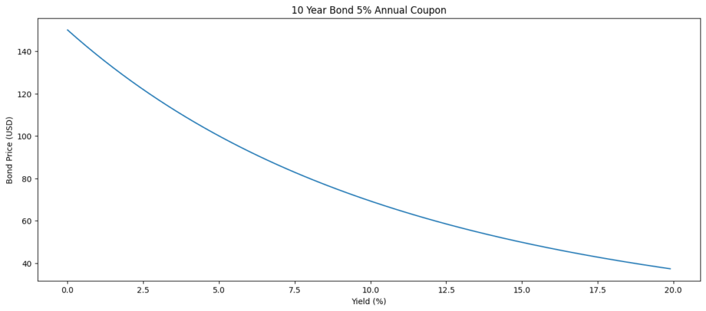
We can visualize the relationship between the price (USD) and the yield (%) for a 10-year bond with an annual 5% coupon in the Python code below.
#########################################################
# BOND PRICES VS. YIELD
#########################################################

# Import necessary libraries
import numpy as np
import numpy_financial as nfp
import pandas as pd
import matplotlib.pyplot as plt

# Generate a range of bond yields from 0% to 20% in increments of 0.1%
bond_yields = np.arange(0,20,0.1)

# Create a DataFrame to store bond yields
bond = pd.DataFrame(bond_yields,columns=['bond_yields'])
print(bond)

# Calculate the bond prices for a 10-year bond with a 5% annual coupon
bond['bond_price'] = -npf.pv(rate=bond['bond_yields']/100,nper=10,pmt=5,fv=100)

# Create a plot of bond prices versus bond yields
plt.figure(figsize=(15, 6))
plt.plot(bond['bond_yields'],bond['bond_price'])
plt.xlabel('Yield (%)')
plt.ylabel('Bond Price (USD)')
plt.title('10 Year Bond 5% Annual Coupon')

# Display the plot
plt.show()
In the visualization above, we can see an inverse relationship between the bond price and the yield. When the bond has a higher price, it lowers the return on investment (yield). A bond is priced at a premium if the price is above $100, at a discount if priced below $100, and at par is priced exactly at $100.
Interest Rate Sensitivity
Coupon rates and interest rates are correlated because changes in market interest rates impact the attractiveness of fixed coupon payments, leading to price adjustments in the bond market to maintain competitive yields.
or example, consider two bonds, one with a 5-year maturity and another with a 10-year maturity, both having a 5% coupon rate. When the yield is 5%, their prices are both $100. Now, let’s observe how their prices are affected by a 6% interest rate.
#########################################################
# INTEREST RATE SENSITIVITY
#########################################################

### 5 YEAR BOND

# 5-year bond
-npf.pv(rate=0.05, nper=5, pmt=5, fv=100)
----------------- OUTPUT -----------------------
100
------------------------------------------------

# 5-year bond with 6% interst rate
-npf.pv(rate=0.06, nper=5, pmt=5, fv=100)
----------------- OUTPUT -----------------------
95.78763621443429
------------------------------------------------

### 10 YEAR BOND

# 10-year bond
-npf.pv(rate=0.05, nper=10, pmt=5, fv=100)
----------------- OUTPUT -----------------------
100
------------------------------------------------

# 10-year bond with 6% interst rate
-npf.pv(rate=0.06, nper=10, pmt=5, fv=100)
----------------- OUTPUT -----------------------
92.63991294858529
------------------------------------------------
As shown above, when the interest rate increases to 6%, the 5-year bond declines to 95.79 (a loss of 4.21% in value), whereas the 10-year bond drops to 92.64 (a loss of 7.36% in value). This demonstrates that the 10-year bond is more sensitive to changes in interest rates.
Duration
Duration is a key concept in bond analysis that measures the sensitivity of a bond’s price to changes in interest rates. It is a useful metric for bond investors and portfolio managers to assess the risk associated with interest rate movements.
Duration quantifies how much a bond’s price is expected to change for a 1% change in interest rates. It measures the bond’s price risk due to interest rate fluctuations. Longer duration implies greater price sensitivity to interest rate changes, while shorter duration suggests less sensitivity.
#########################################################
# DURATION
#########################################################

# Calculate the PV of a bond with a 5% interest rate, 10-year maturity,
price = -npf.pv(rate=0.05, nper=10, pmt=5, fv=100)

# Calculate the PV of the same bond with an interest rate of 6%.
price_up = -npf.pv(rate=0.06, nper=10, pmt=5, fv=100)

# Calculate the PV of the same bond with an interest rate of 4%.
price_down = -npf.pv(rate=0.04, nper=10, pmt=5, fv=100)

# Calculate the duration of the bond
duration = (price_down - price_up) / (2 * price * 0.01)

# Print the calculated duration.
print("Duration:", duration)

----------------- OUTPUT -----------------------
Duration: 7.735491415384871
------------------------------------------------
As seen above, a 1% move in the interest rate causes a 7.74% change in the bond price.
Bond Maturity Against Duration
Bond Maturity:
- Bond maturity refers to the length of time until the bond issuer repays the principal amount to the bondholder. It is the date on which the face value of the bond is returned to the investor, and the bond ceases to exist.
Bond Duration:
- Bond duration is a measure of a bond’s interest rate sensitivity or price sensitivity to changes in interest rates. It takes into account both the bond’s coupon payments and the return of principal at maturity.
The relationship between bond maturity and duration can be summarized as follows:
Short-Term Bonds:
- Short-term bonds generally have shorter durations. Their prices are less sensitive to changes in interest rates because the return on principal is relatively sooner. While short-term bonds may be less sensitive to interest rate movements, they still can be affected by changes in short-term interest rates.
Long-Term Bonds:
- Long-term bonds typically have longer durations. They are more sensitive to changes in interest rates because the return on principal is further into the future. Consequently, long-term bonds are more exposed to interest rate risk.
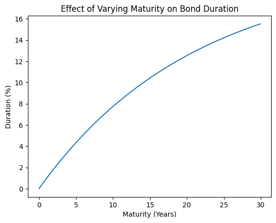
We can plot the relationship between the bond maturity and the duration:
#########################################################
# BOND MATURITY AGAINST DURATION
#########################################################

import numpy as np
import numpy_financial as npf
import pandas as pd
import matplotlib.pyplot as plt

# Generate an array of bond maturities ranging from 0 to 30 years with a step of 0.1 year
bond_maturity = np.arange(0,30,0.1)

# Create a pandas DataFrame to store bond maturity and related calculations
bond = pd.DataFrame(bond_maturity, columns=['bond_maturity'])

# Calculate the bond prices for different maturities, assuming a 5% interest rate, $5 coupon payments, and a face value of $100
bond['price'] = -npf.pv(rate=0.05, nper=bond['bond_maturity'],pmt=5,fv=100)

# Calculate bond prices for scenarios with a 1% increase and a 1% decrease in interest rates
bond['price_up'] = -npf.pv(rate=0.05 + 0.01, nper=bond['bond_maturity'], pmt=5, fv=100)
bond['price_down'] = -npf.pv(rate=0.05 - 0.01, nper=bond['bond_maturity'],pmt=5, fv=100)

# Calculate Macaulay duration for each maturity, representing the sensitivity of bond prices to interest rate changes
bond['duration'] = (bond['price_down'] - bond['price_up']) / (2*bond['price']*0.01)

# Plot the relationship between bond maturity and duration
plt.plot(bond['bond_maturity'],bond['duration'])
plt.xlabel('Maturity (Years)')
plt.ylabel('Duration (%)')
plt.title('Effect of Varying Maturity on Bond Duration')
plt.show()
As seen in the chart above, as the maturity (years) increases, the duration (%) also increases because long-term bonds are more exposed to interest rate risk.
Convexity
Convexity is a measure of the curvature or the degree of curvature in the relationship between a bond’s price and its yield. It is an important concept in fixed-income securities, providing additional insight into how a bond’s price changes in response to fluctuations in interest rates.
When we discuss bond prices and interest rates, there’s an inverse relationship: as interest rates rise, bond prices generally fall, and vice versa. However, this relationship is not perfectly linear. Convexity takes into account the curvature of this price-yield relationship, offering a more accurate description than duration alone.
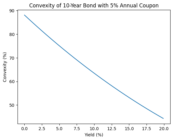
The Python code below shows the relationship between convexity (%) and yield (%):
#########################################################
# YIELD VS. CONVEXITY
#########################################################

# Generate an array of bond yields ranging from 0% to 20% with a step of 0.1%
bond_yields = np.arange(0, 20, 0.1)

# Create a pandas DataFrame to store bond yields and related calculations
bond = pd.DataFrame(bond_yields, columns=['bond_yield'])

# Calculate bond prices for different yields, assuming a 10-year maturity, $5 annual coupon payments, and a face value of $100
bond['price'] = -npf.pv(rate=bond['bond_yield'] / 100, nper=10, pmt=5, fv=100)

# Calculate bond prices for scenarios with a 1% increase and a 1% decrease in yields
bond['price_up'] = -npf.pv(rate=bond['bond_yield'] / 100 + 0.01, nper=10, pmt=5, fv=100)
bond['price_down'] = -npf.pv(rate=bond['bond_yield'] / 100 - 0.01, nper=10, pmt=5, fv=100)

# Calculate convexity for each yield, representing the curvature in the price-yield relationship
bond['convexity'] = (bond['price_down'] + bond['price_up'] - 2 * bond['price']) / (bond['price'] * 0.01 ** 2)

# Plot the relationship between bond yield and convexity
plt.plot(bond['bond_yield'], bond['convexity'])
plt.xlabel('Yield (%)')
plt.ylabel('Convexity (%)')
plt.title('Convexity of 10-Year Bond with 5% Annual Coupon')
plt.show()
The plot shows convexity (%) declining as yields (%) increase illustrating an important characteristic of bond pricing and interest rate sensitivity. The decline in convexity suggests that the bond’s price-yield relationship becomes less curved as yields rise. In other words, the bond becomes less sensitive to interest rate changes in terms of curvature. Lower convexity can be associated with lower price volatility in response to interest rate changes. While lower convexity may reduce price volatility in response to interest rate changes, it also means that investors might experience smaller gains when interest rates fall and smaller losses when interest rates rise compared to bonds with higher convexity.
Conclusion
In this exploration of TVM and bond analysis with Python, we’ve demystified financial complexities using concise code snippets. Python’s dynamic capabilities empower us to navigate compound interest, financial functions, and bond calculations seamlessly.
References
- Bond Valuation and Analysis in Python on DataCamp by Hadrien Lacroix.
- Investopedia. How to Evaluate Bond Performance.
- Fidelity. Fixed Income Analysis Tool.