Backtesting

Backtesting is a critical process in finance that involves testing the performance of a trading or investment strategy using historical data. It provides valuable insights into how a trading or investment strategy might have performed in the past.

Trading signals are commonly used in backtesting as an essential part of evaluating the performance of a trading strategy. To learn more about different types of trading signals, check out my post about Financial Indicators.

Backtesting Process

Backtesting is a systematic process and involves the following 10 key steps:

1. Strategy Formulation: Defining the trading or investment strategy, which could include specific rules and criteria for making buy or sell decisions, using technical indicators, fundamental analysis, or a combination of factors to generate trading signals. For instance, a trading signal could be when the stock price rises above the SMA (Simple Moving Average).
2. Data Collection: Gathering historical data, such as historical price information, trading volumes, and other relevant data points.
3. Data Preprocessing: Cleaning and preprocessing the historical data to ensure it is consistent and free from errors. The quality and accuracy of historical data are crucial for reliable backtesting.
4. Backtest Simulation: Applying the trading strategy to the historical data as if it were being executed in real-time.
5. Portfolio Management: Tracking the hypothetical portfolio’s performance during the backtest. This could include managing position sizes, accounting for transaction costs, and implementing risk management techniques.
6. Performance Metrics: Calculating various performance metrics to evaluate the strategy’s performance. Common metrics include:
   • Total Return: The cumulative profit or loss over the backtest period.
   • Risk-Adjusted Return: Measures like the Sharpe ratio or Sortino radio.
   • Maximum Drawdown: The largest peak-to-through decline in portfolio value.
   • Win-Loss Ratio: The ratio of winning trades to losing trades.
   • Risk Metrics: Metrics that access risk, such as standard deviation or volatility.
7. Out-of-Sample Testing: Reserving a portion of the historical data for out-of-sample testing, and is used to validate the strategy’s performance on unseen data.
8. Analysis and Optimization: Identify strengths and weaknesses, and consider making adjustments or optimization to improve performance.
9. Forward Testing: If the backtest results are satisfactory, deploy the strategy in a forward-testing environment to assess its performance in real-time conditions.
10. Continuous Monitoring: After deployment, continue to monitor the strategy’s performance in live trading, and make necessary adjustments as market conditions change.

Backtesting Strategies in Python

Example #1: SMA/EMA Signal-Based Strategy

This Python code implements a backtesting strategy for Google’s stock price. It initiates a long position when the stock price surpasses the 20-day Simple Moving Average (SMA) and the 20-day Exponential Moving Average (EMA), allowing for a comparison between these two moving averages.

# Import Libraries
import pandas as pd
import bt
import talib
import matplotlib.pyplot as plt

############################################
# STEP 1: IMPORTING DATA & DATA FORMATTING
############################################

# Define the ticker symbol for Google (GOOGL)
ticker_symbol = 'GOOGL'

# Fetch historical data for the stock
price_data = bt.get(ticker_symbol, start='2020-1-1', end='2023-7-31')

############################################
# STEP 2: SIMPLE MOVING AVERAGE (SMA)
############################################

# Calculate the SMA
sma = price_data.rolling(20).mean()

############################################
# STEP 3: EXPONENTIAL MOVING AVERAGE (EMA)
############################################

# Calculate the EMA
ema = price_data.ewm(span=20, adjust=False).mean()

############################################
# STEP 4: DEFINE STRATEGIES
############################################

# Define the SMA strategy
bt_sma_strategy = bt.Strategy('AboveSMA',
                              [bt.algos.SelectWhere(price_data > sma),
                               bt.algos.WeighEqually(),
                               bt.algos.Rebalance()])

# Define the EMA strategy
bt_ema_strategy = bt.Strategy('AboveEMA',
                              [bt.algos.SelectWhere(price_data > ema),
                               bt.algos.WeighEqually(),
                               bt.algos.Rebalance()])

# Create the backtests and run them
bt_sma_backtest = bt.Backtest(bt_sma_strategy, price_data)
bt_ema_backtest = bt.Backtest(bt_ema_strategy, price_data)
bt_sma_result = bt.run(bt_sma_backtest)
bt_ema_result = bt.run(bt_ema_backtest)

############################################
# STEP 5: PLOTTING DATA
############################################

# Create a single subplot
fig, ax1 = plt.subplots(figsize=(15, 8))

# Plot the backtest results on the subplot (ax1)
bt_sma_result.plot(title='SMA vs. EMA Backtest Result', ax=ax1)
bt_ema_result.plot(ax=ax1)

# Add an annotation with the last value for SMA on ax1
last_sma_date = bt_sma_result.prices.index[-1]
last_sma_values = bt_sma_result.prices.iloc[-1, :]
for idx, val in enumerate(last_sma_values.index):
    plt.annotate(f'SMA {val}: {last_sma_values[idx]:.2f}', xy=(last_sma_date, last_sma_values[idx]), xytext=(-30, 5), textcoords='offset points', fontsize=12)

# Add an annotation with the last value for EMA on ax1
last_ema_date = bt_ema_result.prices.index[-1]
last_ema_values = bt_ema_result.prices.iloc[-1, :]
for idx, val in enumerate(last_ema_values.index):
    plt.annotate(f'EMA {val}: {last_ema_values[idx]:.2f}', xy=(last_ema_date, last_ema_values[idx]), xytext=(-30, 5), textcoords='offset points', fontsize=12)

# Add a legend
ax1.legend()

plt.show()

Example #2: Trend Following Strategies

This Python code implements a backtesting strategy for Google’s stock price and initiates a long signal when the short-term EMA crosses above the long-term EMA and a short signal when the short-term EMA crosses below the long-term EMA.

# Import Libraries
import pandas as pd
import bt
import talib
import matplotlib.pyplot as plt

############################################
# STEP 1: IMPORTING DATA & DATA FORMATTING
############################################

# Define the ticker symbol for Google (GOOGL)
ticker_symbol = 'GOOGL'

# Fetch historical data for the stock
price_data = bt.get(ticker_symbol, start='2020-1-1', end='2023-7-31')

############################################
# STEP 2: CALCULATE THE INDICATORS (EMA 20 & 40)
############################################

# Calculate the EMA
EMA_short = price_data.ewm(span=20, adjust=False).mean()
EMA_long = price_data.ewm(span=40, adjust=False).mean()

############################################
# STEP 3: CONSTRUCT THE SIGNAL
############################################

# Create the signal DataFrame
signal = EMA_long.copy()
 
signal[EMA_long.isnull()] = 0
 
# Construct the signal
signal[EMA_short > EMA_long] = 1
signal[EMA_short <= EMA_long] = -1

# Merge the data 
combined_df = bt.merge(signal, price_data, EMA_short, EMA_long)
combined_df.columns = ['signal', 'Price', 'EMA_short', 'EMA_long']

############################################
# STEP 4: PLOTTING DATA
############################################

# Plot the signal, price and MAs
combined_df.plot(secondary_y=['signal'], figsize=(15, 8))

plt.show()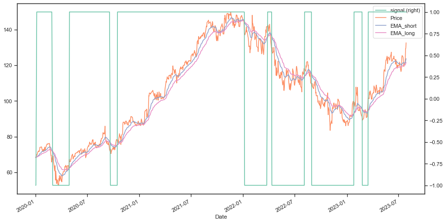

Python Code Continued…

############################################
# STEP 5: DEFINE THE STRATEGY
############################################

# Define the strategy
bt_strategy = bt.Strategy('EMA_crossover', 
                          [bt.algos.WeighTarget(signal),
                           bt.algos.Rebalance()])

# Create the backtest and run it
bt_backtest = bt.Backtest(bt_strategy, price_data)
bt_result = bt.run(bt_backtest)

############################################
# STEP 6: PLOTTING THE RESULT
############################################

# Plot the backtest result
bt_result.plot(title='Backtest result')

# Add an annotation with the last value
last_date = bt_result.prices.index[-1]
last_value = bt_result.prices.iloc[-1, -1]
plt.annotate(f' {last_value:.2f}', xy=(last_date, last_value), xytext=(-30, 5), textcoords='offset points', fontsize=12)

plt.show()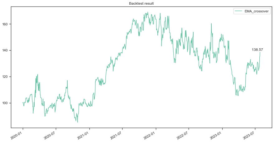

Example #3: Mean Reversion Strategy

The Python code below implements a mean reversion strategy using the Relative Strength Index (RSI):

• Short Signal: RSI > 70
  • Suggests the asset is likely overbought and the price may soon reverse.
• Long Signal: RSI < 30
  • Suggests the asset is likely oversold and the price may soon rally.

This RSI-based mean reversion strategy tries to take advantage of temporary market imbalances and trades more frequently.

# Import Libraries
import pandas as pd
import bt
import talib
import matplotlib.pyplot as plt

############################################
# STEP 1: IMPORTING DATA & DATA FORMATTING
############################################


# Define the ticker symbol for Google (GOOGL)
ticker_symbol = 'GOOGL'

# Fetch historical data for the stock
price_data = bt.get(ticker_symbol, start='2020-1-1', end='2023-7-31')

############################################
# STEP 2: CALCULATE RSI
############################################

# Calculate the RSI
stock_rsi = talib.RSI(price_data['googl']).to_frame()

############################################
# STEP 3: CONSTRUCT THE SIGNAL
############################################

# Create the same DataFrame structure as RSI
signal = stock_rsi.copy()
signal[stock_rsi.isnull()] = 0

# Construct the signal
signal[stock_rsi < 30] = 1
signal[stock_rsi > 70] = -1
signal[(stock_rsi <= 70) & (stock_rsi >= 30)] = 0

signal.rename(columns={0: 'googl'}, inplace=True)


############################################
# STEP 4: DEFINE THE STRATEGY
############################################

# Define the strategy
bt_strategy = bt.Strategy('RSI_MeanReversion', 
                          [bt.algos.WeighTarget(signal),
                           bt.algos.Rebalance()])


# Create the backtest and run it
bt_backtest = bt.Backtest(bt_strategy, price_data)
bt_result = bt.run(bt_backtest)

############################################
# STEP 5: PLOTTING DATA
############################################

# Plot the backtest result
bt_result.plot(title='Backtest result', figsize=(15, 8))

# Add an annotation with the last value
last_date = bt_result.prices.index[-1]
last_value = bt_result.prices.iloc[-1, -1]
plt.annotate(f' {last_value:.2f}', xy=(last_date, last_value), xytext=(-30, 5), textcoords='offset points', fontsize=12)

plt.show()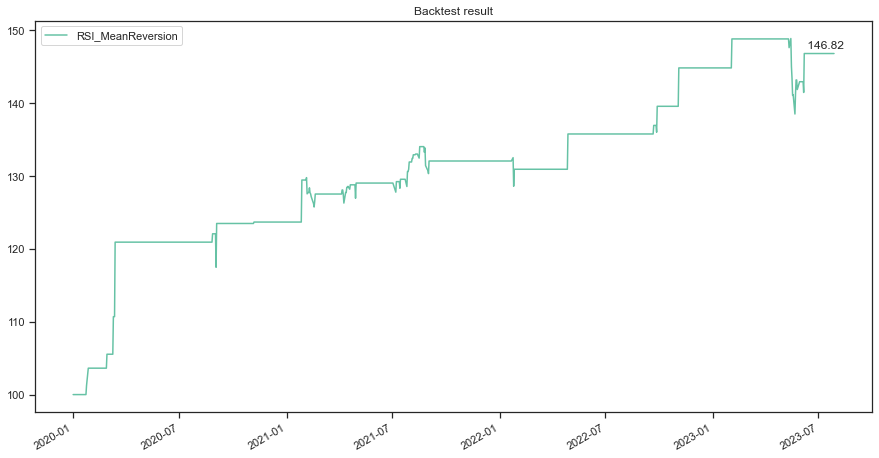

Backtesting Results and Performance Summary

• Signal-Based Strategy
  • 20-Day SMA Signal-Based Strategy: 154.04 🥈
  • 20-Day EMA Signal-Based Strategy: 168.56 🥇
• Trend Following Strategies:
  • Short-term EMA crosses above the long-term EMA: 138.37
• Mean Reversion Strategy:
  • Relative Strength Index (RSI): 146.82 🥉

Based on the summary results provided above, it’s evident that the Signal-Based Strategy utilizing the 20-day EMA delivered the highest profitability. But is the 20-day lockback period the best period? In the section below I will describe strategy optimization and benchmarking.

Strategy Optimization and Benchmarking

Strategy Optimization

Strategy optimization involves experimenting with various input parameter values during backtesting and then comparing the resulting outcomes. For instance, for signal-based strategy, is EMA 20-day, 30-day, or 40-day better?

The Python code below compares the following three strategies:

1. Initiates a long position when Google’s stock price surpasses the 20-day Simple Moving Average
2. Initiates a long position when Google’s stock price surpasses the 30-day Simple Moving Average
3. Initiates a long position when Google’s stock price surpasses the 50-day Simple Moving Average

# Import Libraries
import pandas as pd
import bt
import talib
import matplotlib.pyplot as plt

############################################
# STEP 1: IMPORTING DATA & DATA FORMATTING
############################################

# Define the ticker symbol for Google (GOOGL)
ticker_symbol = 'GOOGL'

# Fetch historical data for the stock
price_data = bt.get(ticker_symbol, start='2020-1-1', end='2023-7-31')

############################################
# STEP 2: SIMPLE MOVING AVERAGE (SMA)
############################################

def signal_strategy(price_data, period, name):
    # Calculate SMA
    sma = price_data.rolling(period).mean()
    # Define the signal-based Strategy
    bt_strategy = bt.Strategy(name, 
                              [bt.algos.SelectWhere(price_data>sma),
                               bt.algos.WeighEqually(),
                               bt.algos.Rebalance()])
    # Return the backtest
    return bt.Backtest(bt_strategy, price_data)

############################################
# STEP 3: SIGNAL STRATEGY USING DIFFERENT SMAs
############################################


# Create signal strategy backtest
sma10 = signal_strategy(price_data, period=10, name='SMA10')
sma30 = signal_strategy(price_data, period=30, name='SMA30')
sma50 = signal_strategy(price_data, period=50, name='SMA50')

# Run all backtests and plot the resutls
bt_results = bt.run(sma10, sma30, sma50)

############################################
# STEP 4: PLOTTING THE RESULT
############################################

# Plot the backtest result
bt_results.plot(title='Strategy Optimization', figsize=(15, 8))

plt.show()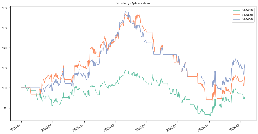

Benchmarking

Benchmarking in backtesting refers to comparing the performance of a trading or investment strategy against a benchmark or a reference point. The benchmark is typically a standard or widely recognized index, asset, or portfolio that represents a relevant market or asset class. By benchmarking a strategy, it is possible to assess how well it performs in comparison.

For instance, the S&P 500 Index is often used as a benchmark for equities, while the U.S. Treasuries are used for measuring bond risks and returns.

The Python code below shows the stock price if it was bought on 1/1/2020 and not sold, as a benchmark, and then compared to the three signal-trading strategies above (SMA 10, 30, and 50).

# Import Libraries
import pandas as pd
import bt
import talib
import matplotlib.pyplot as plt

############################################
# STEP 1: IMPORTING DATA & DATA FORMATTING
############################################

# Define the ticker symbol for Google (GOOGL)
ticker_symbol = 'GOOGL'

# Fetch historical data for the stock
price_data = bt.get(ticker_symbol, start='2020-1-1', end='2023-7-31')

############################################
# STEP 2: BENCHMARKING
############################################

# The following code shows the stock price if it was bought on 
# 1/1/2020 and hold since then.

def buy_and_hold(price_data, name):
    # Define the benchmark strategy
    bt_strategy = bt.Strategy(name, 
                              [bt.algos.RunOnce(),
                               bt.algos.SelectAll(),
                               bt.algos.WeighEqually(),
                               bt.algos.Rebalance()])
    # Return the backtest
    return bt.Backtest(bt_strategy, price_data)

# Create benchmark strategy backtest
benchmark = buy_and_hold(price_data, name='benchmark')

# Run all backtests and plot the resutls
bt_results = bt.run(sma10, sma30, sma50, benchmark)

############################################
# STEP 3: PLOTTING THE RESULT
############################################

bt_results.plot(title='Strategy benchmarking', figsize=(15, 8))
plt.show()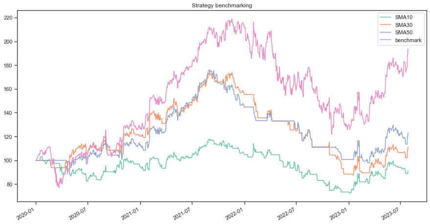

Conclusion

Backtesting, strategy optimization, and benchmarking are essential tools in the realm of investment and trading. They allow investors and traders to rigorously assess the performance of their strategies, refine them for better results, and compare them against established benchmarks.

Backtesting serves as the foundation of strategy evaluation by simulating historical trading scenarios. It enables traders and investors to understand how their strategies would have performed in the past, providing a historical context for decision-making.

Strategy optimization is the iterative process of fine-tuning a trading or investment strategy by adjusting its parameters or rules. Optimization aims to enhance a strategy’s risk-adjusted returns and overall effectiveness.

Benchmarking allows investors and traders to put their strategies into context by comparing them to established benchmarks or reference points. These benchmarks represent the performance of passive investment strategies or market indices.

In some cases, such as the one above, passive strategies such as investing and holding the stock can outperform active trading strategies.